Plotting Maps
Maps for geospatial data, such as EarthCARE orbital tracks or MSI swath data, can be created using the cartopy-based MapFigure class.
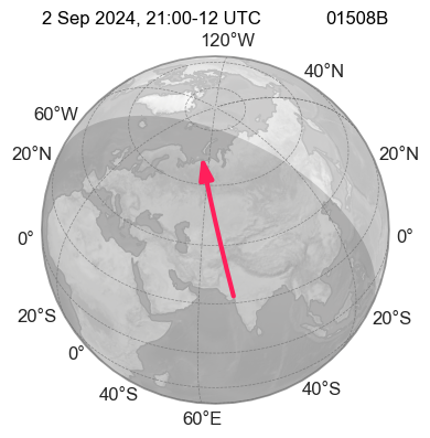
Orbital tracks of EarthCARE datasets
Like the other earthcarekit figure classes, MapFigure also has the ecplot method, which enables plotting directly from an open EarthCARE dataset.
import earthcarekit as eck

df = eck.search_product(file_type="AEBD", orbit_and_frame="01508B")
fp = df.filepath[-1]  # ECA_EXBB_ATL_EBD_2A_20240902T210023Z_20251107T142547Z_01508B.h5

with eck.read_product(fp) as ds:
    mfig = eck.MapFigure()
    mfig.ecplot(ds)
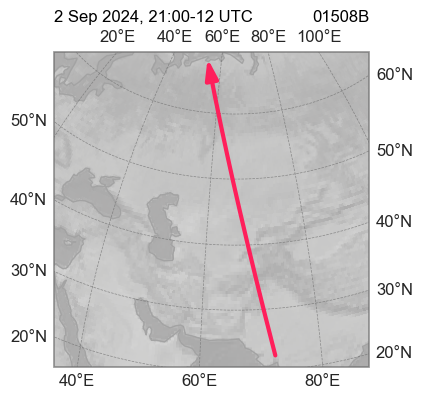
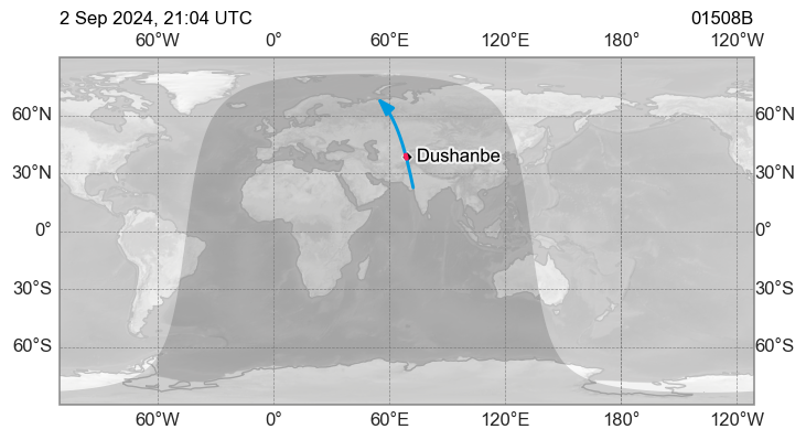
To zoom in on the relevant area where the data is located, the argument view can be set to "data".
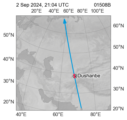
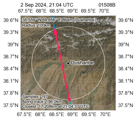
In this example, we use an EarthCARE frame from a overpass of the ground site at Dushanbe, Tajikistan. To visualise this on the map, the location (and optionally the radius, by default 100 km) can be specified.
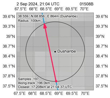
For overpasses, the view option can be set to "overpass" to zoom in on data within the specified radius and display additional information about the overpass event as text.
To change the background image of the globe, the style arguement can be changed in the MapFigure constructor. Here, layer names from Web Map Services (WMS) can also be used to retrieve images from either EUMETSAT's EUMETView WMS or NASA's Global Imagery Browse Service (GIBS).
For example, "blue_marble" will fetch the "BlueMarble_ShadedRelief_Bathymetry" image layer from the NASA GIBS WMS:
Instead of the default orthographic projection, a lat/lon or plate carrée projection can be used.
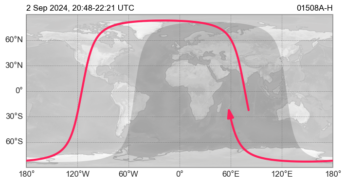
In this example, an entire orbit track is plotted:
eck.ecdownload(file_type="ACTH:BA", orbit_number=1508, verbose=False)

df = eck.search_product(file_type="ACTH:BA", orbit_number=1508).filter_latest()

with eck.read_products(df) as ds:
    mfig = eck.MapFigure(
        projection="platecarree",
        fig_width_scale=2,
        show_top_labels=False,
        show_right_labels=False
    )
    mfig.ecplot(ds, central_longitude=0)
See content of df variable ...
| mission_id | agency | latency | baseline | file_type | start_sensing_time | start_processing_time | orbit_number | frame_id | orbit_and_frame | name | filepath | hdr_filepath | |
|---|---|---|---|---|---|---|---|---|---|---|---|---|---|
| 0 | ECA | E | X | BA | ATL_CTH_2A | 2024-09-02 20:48:48 | 2025-09-06 22:36:51 | 1508 | A | 01508A | ECA_EXBA_ATL_CTH_2A_20240902T204848Z_20250906T223651Z_01508A | ... | ... |
| 1 | ECA | E | X | BA | ATL_CTH_2A | 2024-09-02 21:00:23 | 2025-07-21 13:51:46 | 1508 | B | 01508B | ECA_EXBA_ATL_CTH_2A_20240902T210023Z_20250721T135146Z_01508B | ... | ... |
| 2 | ECA | E | X | BA | ATL_CTH_2A | 2024-09-02 21:12:10 | 2025-09-06 22:27:32 | 1508 | C | 01508C | ECA_EXBA_ATL_CTH_2A_20240902T211210Z_20250906T222732Z_01508C | ... | ... |
| 3 | ECA | E | X | BA | ATL_CTH_2A | 2024-09-02 21:23:14 | 2025-09-06 22:28:58 | 1508 | D | 01508D | ECA_EXBA_ATL_CTH_2A_20240902T212314Z_20250906T222858Z_01508D | ... | ... |
| 4 | ECA | E | X | BA | ATL_CTH_2A | 2024-09-02 21:35:00 | 2025-09-06 22:09:27 | 1508 | E | 01508E | ECA_EXBA_ATL_CTH_2A_20240902T213500Z_20250906T220927Z_01508E | ... | ... |
| 5 | ECA | E | X | BA | ATL_CTH_2A | 2024-09-02 21:46:35 | 2025-09-06 22:34:06 | 1508 | F | 01508F | ECA_EXBA_ATL_CTH_2A_20240902T214635Z_20250906T223406Z_01508F | ... | ... |
| 6 | ECA | E | X | BA | ATL_CTH_2A | 2024-09-02 21:58:23 | 2025-09-06 22:34:05 | 1508 | G | 01508G | ECA_EXBA_ATL_CTH_2A_20240902T215823Z_20250906T223405Z_01508G | ... | ... |
| 7 | ECA | E | X | BA | ATL_CTH_2A | 2024-09-02 22:09:30 | 2025-09-06 22:14:17 | 1508 | H | 01508H | ECA_EXBA_ATL_CTH_2A_20240902T220930Z_20250906T221417Z_01508H | ... | ... |
MSI swath data
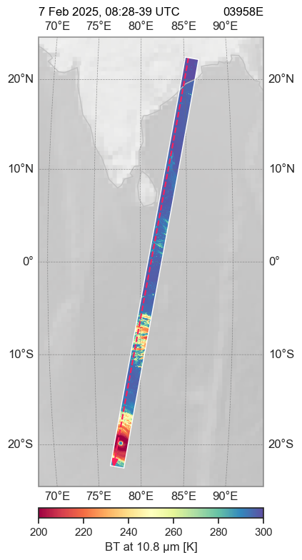
If the EarthCARE dataset used contains swath data, this can be displayed on the map by specifying the corresponding variable name (var):
df = eck.search_product(file_type="MRGR", orbit_and_frame="03958E")
fp = df.filepath[-1]  # ECA_EXBA_MSI_RGR_1C_20250207T082755Z_20250623T011250Z_03958E.h5

with eck.read_product(fp) as ds:
    mfig = eck.MapFigure(fig_height_scale=2)
    mfig.ecplot(ds, var="tir2", view="data", value_range=(200, 300), cmap="Spectral")
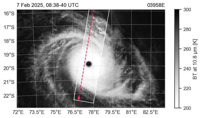
Using the options zoom_tmin, zoom_tmax and setting view="overpass", you can zoom in on a specific time period of the overpass, without having to define a ground site and radius.
mfig = eck.MapFigure(
    style="msg_iodc:ir108",  # Retrieves background image from EUMENTView
    show_top_labels=False,
    show_right_labels=False,
    grid_color="lightgray",
    fig_width_scale=1.5,
)
mfig.ecplot(
    ds=ds,
    var="tir2",
    value_range=(200, 300),
    colorbar_position="right",
    zoom_tmin="20250207T0838",  # Time period to be zoomed in on
    zoom_tmax="20250207T0840",  # Time period to be zoomed in on
    view="overpass",            # Time period to be zoomed in on
)
Manual plotting including non-EarthCARE geospacial data
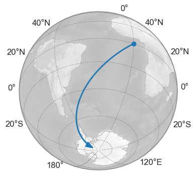
In addition to ecplot, there are other class methods that enable the plotting of non-EarthCARE data, for example using numpy arrays.
# Generating example data
x = np.linspace(0, 1, 100)
lats = x * -85
lons = x * -85

mfig = eck.MapFigure(central_latitude=lats, central_longitude=lons)
mfig.plot_track(latitude=lats, longitude=lons)
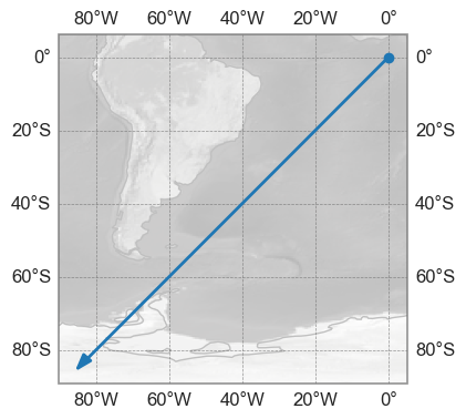
Also, here the same data using the plate carrée projection and zoomed in on the lat/lon data:
mfig = eck.MapFigure(central_latitude=lats, central_longitude=lons, projection="platecarree")
mfig.plot_track(latitude=lats, longitude=lons)

mfig.set_view(lats, lons)  # Zoom in on data
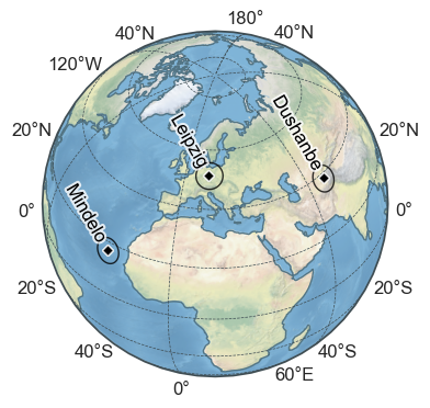
lats = [16.878, 51.352757, 38.559]
lons = [-24.995, 12.43392, 68.856]
names = ["Mindelo", "Leipzig", "Dushanbe"]

mfig = eck.MapFigure(
    central_latitude=lats,
    central_longitude=lons,
    projection="orthographic",
    fig_width_scale=1,
    style="stock_img",
)

for n, lt, ln in zip(names, lats, lons):
    mfig.plot_point(latitude=lt, longitude=ln)
    mfig.plot_radius(latitude=lt, longitude=ln, radius_km=500)
    mfig.plot_text(latitude=lt, longitude=ln, text=n, rotation=-60)
As with the other figure classes, the underlying matplotlib/cartopy axes of each figure can be accessed from the [MapFigure.ax][earthcarekit.MapFigure.ax] property.
This allows standard cartopy to be used to plot your own data.