Plot customizations
Adding or overlaying supplementary data in curtain plots
In this example, the basic curtain plot is created using an A-EBD dataset:
df = eck.search_product(file_type="aebd", orbit_and_frame="01508B")
df = df.filter_latest()
fp = df.filepath[-1] # ECA_EXBA_ATL_EBD_2A_20240902T210023Z_20250721T110708Z_01508B.h5
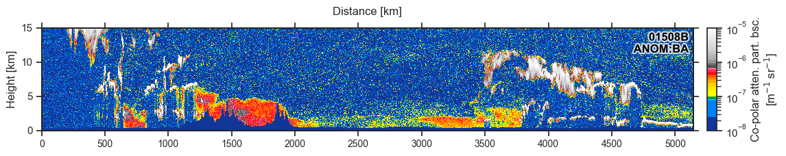
df_anom = eck.search_product(file_type="anom", orbit_and_frame="01508B")
df_anom = df_anom.filter_latest()
fp_anom = df_anom.filepath[-1]
with eck.read_product(fp) as ds:
cf = eck.CurtainFigure(figsize=(9.5, 2.5))
cf.ecplot(ds, var="particle_extinction_coefficient_355nm", height_range=(0, 15e3))

Height data (1D)
One-dimensional height data can be overlayed by using the methods CurtainFigure.ecplot_height when working with datasets or CurtainFigure.plot_height when working with arrays.
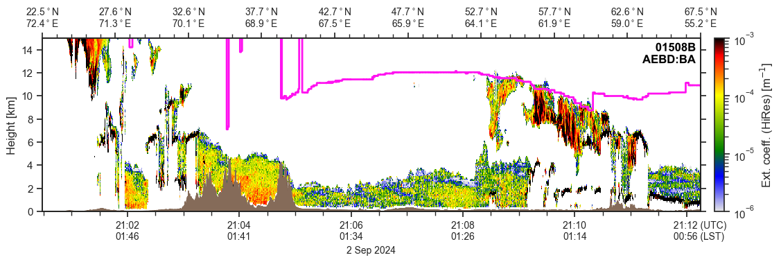
To overlay common height data like the tropopause height or surface elevation, the methods CurtainFigure.ecplot_elevation and CurtainFigure.ecplot_tropopause can be used with datasets that contain the required information (note: here both surface and tropopause information is available in A-EBD):
with eck.read_product(fp) as ds:
    cf = eck.CurtainFigure(figsize=(9.5, 2.5))
    cf.ecplot(ds, var="particle_extinction_coefficient_355nm", height_range=(0, 15e3))
    cf.ecplot_elevation(ds)
    cf.ecplot_tropopause(ds)
Profile data (2D)
To overlay two-dimensional profile data with contour lines the methods CurtainFigure.ecplot_contour (for datasets) or CurtainFigure.plot_contour (for arrays).
To overlay common profile data like the layer temperature or pressure, the methods CurtainFigure.ecplot_temperature and CurtainFigure.ecplot_pressure can be used with datasets that contain the required information (note: since A-EBD does not contain the required data, the related A-NOM product is used for this):
df_anom = eck.search_product(file_type="anom", orbit_and_frame="01508B")
df_anom = df_anom.filter_latest()

fp_anom = df_anom.filepath[-1]  # ECA_EXBA_ATL_NOM_1B_20240902T210023Z_20250630T151754Z_01508B.h5

with (
    eck.read_product(fp) as ds,
    eck.read_product(fp_anom) as ds_anom,
):
    cf = eck.CurtainFigure(figsize=(9.5, 2.5))
    cf.ecplot(ds, var="particle_extinction_coefficient_355nm", height_range=(0, 15e3))
    cf.ecplot_elevation(ds)
    cf.ecplot_tropopause(ds)
    cf.ecplot_temperature(ds_anom)

Also, instead of contours area hatchings can be created using CurtainFigure.ecplot_hatch (for datasets) or CurtainFigure.plot_hatch (for arrays).
In case of A-EBD it can be usefull to visualize the attenuated Lidar signal. This can be done by using the CurtainFigure.ecplot_hatch_attenuated method (note: this requires the "simple_classification" variable stored in A-EBD and other L2 ATLID products)
with eck.read_product(fp) as ds:
    cf = eck.CurtainFigure(figsize=(9.5, 2.5))
    cf.ecplot(ds, var="particle_extinction_coefficient_355nm", height_range=(0, 15e3))
    cf.ecplot_elevation(ds)
    cf.ecplot_tropopause(ds)
    cf.ecplot_hatch_attenuated(ds)

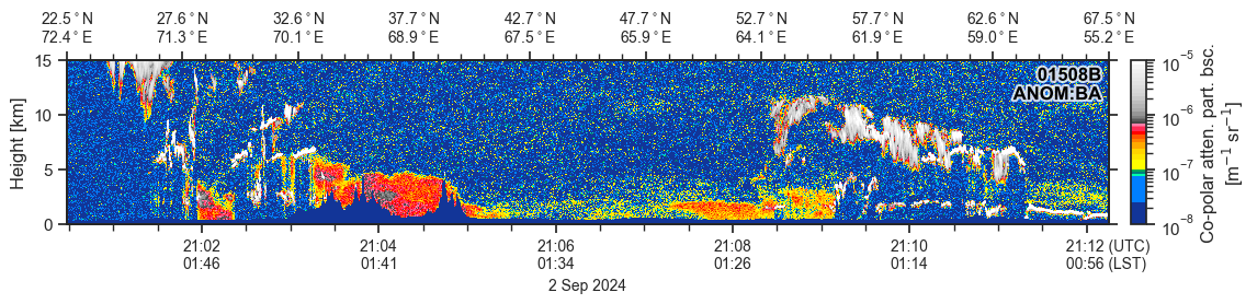
Along-track axis styles
df = eck.search_product(file_type="aebd", orbit_and_frame="01508B")
df = df.filter_latest()

fp = df.filepath[-1]
# fp="path_to/ECA_EXBA_ATL_EBD_2A_20240902T210023Z_20250721T110708Z_01508B.h5"

with eck.read_product(fp) as ds:
    cf = eck.CurtainFigure(
        figsize=(9.5, 1.5),
        ax_style_top="geo",  # default setting
        ax_style_bottom="time",  # default setting
    )
    cf.ecplot(ds, var="mie_attenuated_backscatter", height_range=(0, 15e3))
You can change the displayed axes by setting the ax_style_top and ax_style_bottom arguments. Here are some examples:
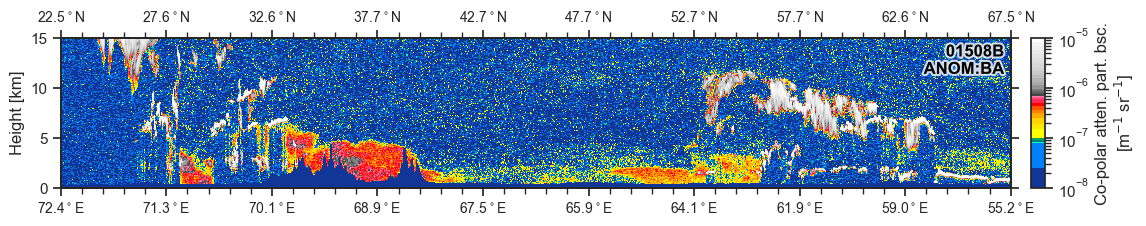
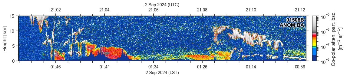

Adding "_nolabels" to the ax_style string removes the tick labels and "_notitle" removes the title (note: both can be used in the same string).
You can also show no labels or change the maximum number of mayor ticks.
