Working with profiles
This tutorial gives an introduction to the ProfileData class and it's use in earthcarekit.
Begin by importing the following modules:
import earthcarekit as eck
import numpy as np
import pandas as pd
The class ProfileData is a container for atmospheric profile data.
It stores profile values together with their time/height bins and, optionally, their coordinates and other metadata (e.g., label and units) in a consistent structure, making profiles easier to handle, compare and visualise.
Overview
ProfileData requires at least three inputs:
- values - the profile data, either of a single vertical profile or a time series of profiles (2D array with time as the first dimension and height as the second).
- height - an array or time series of arrays of ascending height bin centers.
- time - an array of ascending timestamps corresponding to the profiles.
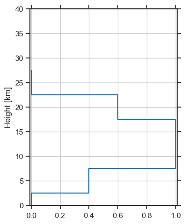
p = eck.ProfileData(
    values=[
        [0, 0.4, 1, 1, 0.6, 0],  # 1 profile (6 bins)
    ],
    height=[0e3, 5e3, 10e3, 15e3, 20e3, 25e3],  # 6 bin centers (can also be 2D if same shape as values)
    time=["2025-01-01T00:00"],  # 1 timestamp for the single profile in values
)
print(p)
See output ...
ProfileData(values=array([[0. , 0.4, 1. , 1. , 0.6, 0. ]]), height=array([ 0., 5000., 10000., 15000., 20000., 25000.]), time=array(['2025-01-01T00:00:00.000000000'], dtype='datetime64[ns]'), latitude=None, longitude=None, color=None, label=None, units=None, platform=None, error=None)
To create a quick plot use the ProfileFigure class:
pf = eck.ProfileFigure().plot(p)
pf.save(filepath="profile1.png")
profile1.png |
 |
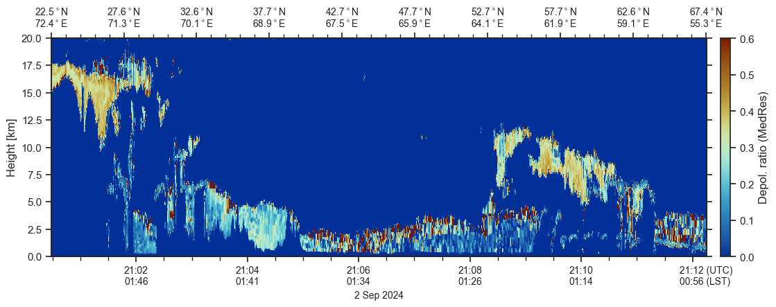
Alternatively, you can initialize a ProfileData object from data stored in a xarray.Dataset, e.g., from a EarthCARE product:
fp = r"./ECA_EXBA_ATL_EBD_2A_20240902T210023Z_20250721T110708Z_01508B.h5" # Replace path with one of your local files
with eck.read_any(fp) as ds:
p_from_ec = eck.ProfileData.from_dataset(
ds=ds,
var="particle_linear_depol_ratio_355nm_medium_resolution", # Select a valid variable from the dataset
)
# Plotting the profile data in a time/height curtain plot
cf = eck.CurtainFigure().plot(p_from_ec, cmap="ratio", value_range=(0, 0.6), height_range=(0, 20e3)) # Custommize curtain plot settings
cf.save(filepath="profile_curtain_from_ec.png")
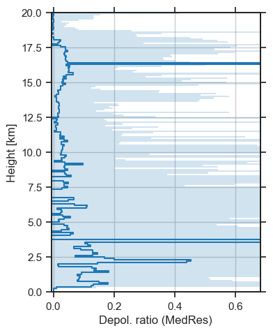
# Plotting the profile (i.e., the mean and STD)
pf = eck.ProfileFigure(height_range=(0, 20e3)).plot(p_from_ec)
pf.save(filepath="profile_from_ec.png")
profile_curtain_from_ec.png |
profile_from_ec.png |
 |
 |
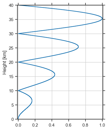
Selection by height range
# Generating example data
nh = 1000  # Number of height bins
h = np.linspace(0, 40e3, nh)  # Height values in meters
v = np.abs(np.sin(np.linspace(np.pi*3, -np.pi, nh)) * h)  # Signal values
v = v / np.max(v)

p = eck.ProfileData(
    values=v,
    height=h,
    time=["2025-01-01T00:00"],
)

# Plotting
pf = eck.ProfileFigure().plot(p)
pf.save(filepath="single_profile1.png")
single_profile1.png |
 |
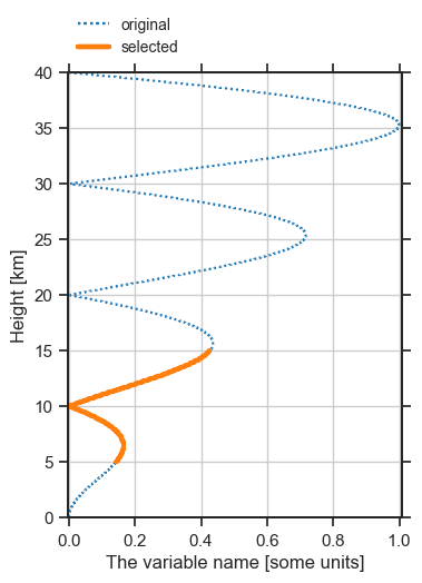
height_range = (5e3, 15e3)  # in meters
p_selected = p.select_height_range(height_range)

# Plotting
pf = eck.ProfileFigure(label="The variable name", units="some units", show_legend=True, value_range=(0, 1))
pf = pf.plot(p, linestyle="dotted", legend_label="original")
pf = pf.plot(p_selected, linewidth=3, legend_label="selected")
pf.save(filepath="single_profile2.png")
single_profile2.png |
 |
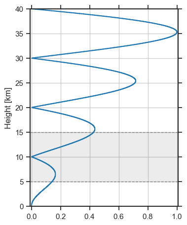
You can also mark the selected height range only in the plot:
pf = eck.ProfileFigure(value_range=(0,1))
pf = pf.plot(p, selection_height_range=(5e3, 15e3))
pf.save(filepath="single_profile3.png")
single_profile3.png |
 |
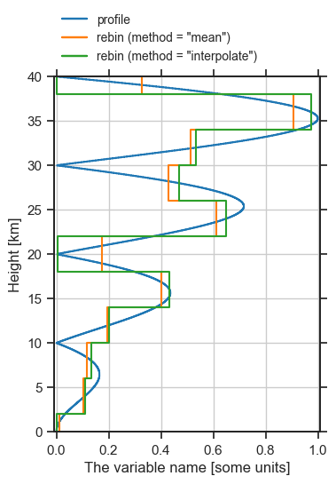
Rebinning
new_height = np.linspace(0, 40e3, 11)  # Generated list of height bin centers

p_rebin_mean = p.rebin_height(new_height)
p_rebin_interp = p.rebin_height(new_height, method="interpolate")

# Plotting
pf = eck.ProfileFigure(label="The variable name", units="some units", show_legend=True, value_range=(0,1))
pf = pf.plot(p, legend_label="profile")
pf = pf.plot(p_rebin_mean, legend_label='rebin (method = "mean")')
pf = pf.plot(p_rebin_interp, legend_label='rebin (method = "interpolate")')
pf.save(filepath="rebinned_profile1.png")
rebinned_profile1.png |
 |
Calculating statistics
results = p.stats()
print(results)
See output ...
ProfileStatResults(hmin=0.0, hmax=40000.0, mean=0.3619352437163005, std=0.2874920456912103, mean_error=None)
results2 = p.stats(height_range=(7_500, 12_500))
results3 = p.stats(height_range=(12_500, 17_500))

# Create a dataframe
df = pd.concat([
    results.to_dataframe(),
    results2.to_dataframe(),
    results3.to_dataframe(),
], ignore_index=True)
|
hmin |
hmax |
mean |
std |
mean_error |
| 0 |
0 |
40000 |
0.361935 |
0.287492 |
nan |
| 1 |
7500 |
12500 |
0.106411 |
0.063519 |
nan |
| 2 |
12500 |
17500 |
0.384492 |
0.0501576 |
nan |
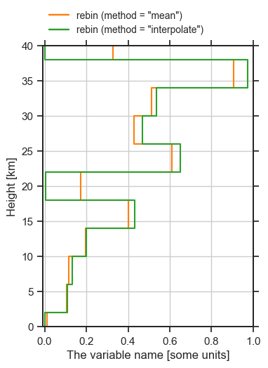
Comparing profiles
We compare the two rebinned profiles from the above section on Rebinning.
Here, p_rebin_mean is the prediction and p_rebin_interp the target.
results = p_rebin_mean.compare_to(p_rebin_interp)
display(results.to_dataframe())  # works only in a Jupyter notebook

# Plotting
pf = eck.ProfileFigure(label="The variable name", units="some units", show_legend=True, value_range=(0,1))
pf = pf.plot(p_rebin_mean, legend_label='rebin (method = "mean")',color="tab:orange")
pf = pf.plot(p_rebin_interp, legend_label='rebin (method = "interpolate")',color="tab:green")
pf.save(filepath="compared_profiles.png")
|
hmin |
hmax |
diff_of_means |
mae |
rmse |
mean_diff |
mean_prediction |
std_prediction |
mean_error_prediction |
mean_target |
std_target |
mean_error_target |
| 0 |
0 |
40000 |
-0.0256926 |
0.0668805 |
0.115323 |
-0.0256926 |
0.344468 |
0.251908 |
nan |
0.318775 |
0.303957 |
nan |
compared_profiles.png |
 |
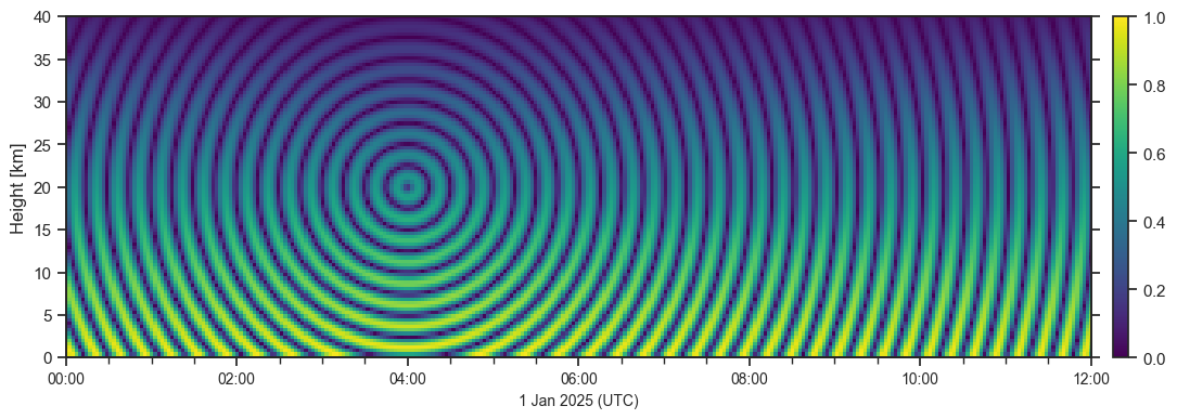
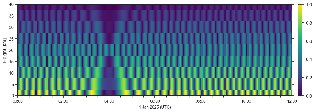
Timeseries of profiles
# Generating example data
nh = 100 # Number of height bins
h = np.linspace(0, 40e3, nh)
nt = 300 # Number of (temporal) samples
y = np.linspace(-0.5, 0.5, nh)
x = np.linspace(-1, 2, nt)
gx, gy = np.meshgrid(x, y)
r = np.sqrt(gx**2 + gy**2)
v = np.sin(50 * r).T
v = np.abs(v) * np.linspace(1, 0.1, nh)
p = eck.ProfileData(
values=v,
height=h,
time=pd.date_range("20250101T00", "20250101T12", periods=nt),
)
# PLotting
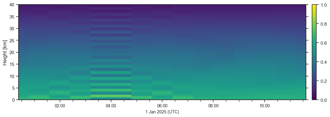
cf = eck.CurtainFigure().plot(p, value_range=(0,1))
cf.save(filepath="ts_curtain.png")
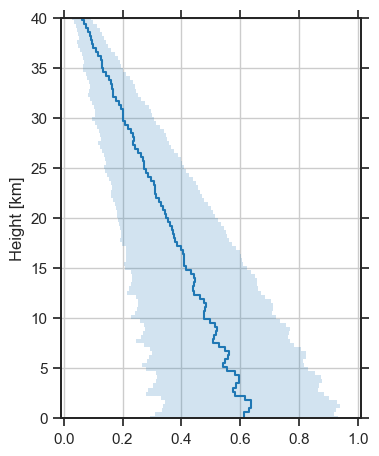
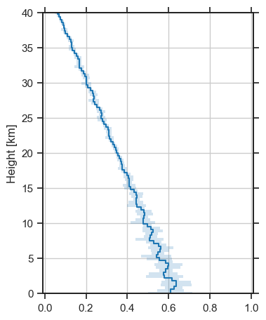
pf = eck.ProfileFigure().plot(p, value_range=(0,1))
pf.save(filepath="ts_profile.png")
ts_curtain.png |
ts_profile.png |
 |
 |
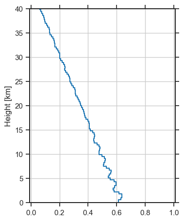
Get the mean profile
p_mean = p.mean()
# p.shape=(300, 100)
# p_mean.shape=(1, 100)

# Plotting
pf = eck.ProfileFigure().plot(p_mean, value_range=(0,1))
pf.save(filepath="ts_mean_profile.png")
ts_mean_profile.png |
 |
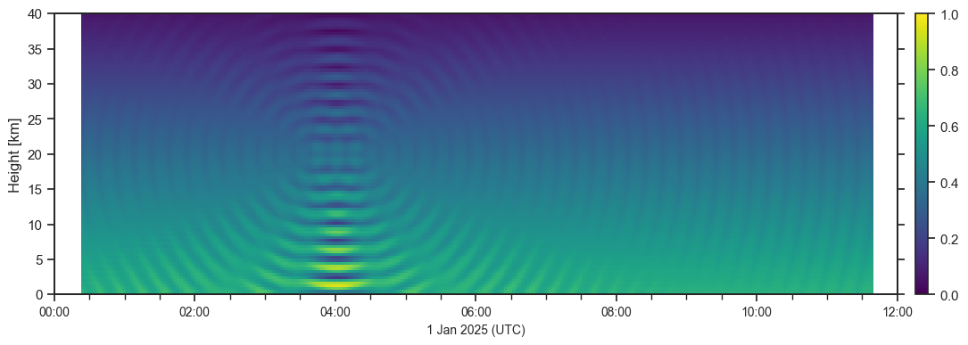
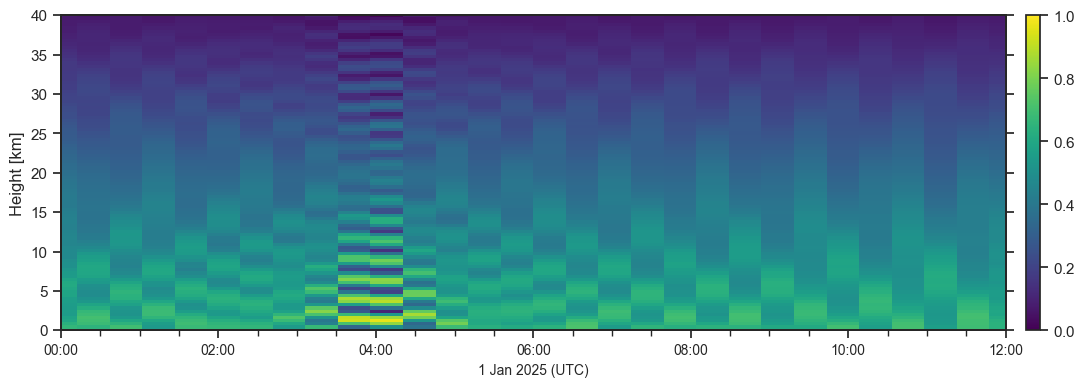
Apply rolling mean (or moving average)
p_roll = p.rolling_mean(20, axis=0)
# p.shape=(300, 100)
# p_roll.shape=(300, 100)

# Plotting
cf = eck.CurtainFigure().plot(p_roll, value_range=(0,1))
pf.save(filepath="ts_rolling_curtain.png")

pf = eck.ProfileFigure().plot(p_roll, value_range=(0,1))
pf.save(filepath="ts_rolling_profile.png")
ts_rolling_curtain.png |
ts_rolling_profile.png |
 |
 |
Coarsen profiles
p_coarsened = p.coarsen_mean(20)
# p.shape=(300, 100)
# p_coarsened.shape=(15, 100)
# Plotting
cf = eck.CurtainFigure().plot(p_coarsened, value_range=(0,1))
cf.save(filepath="ts_coarse_curtain.png")
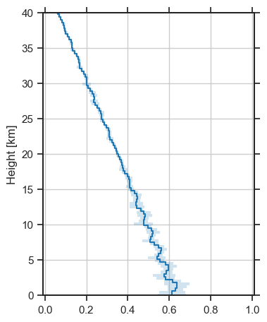
pf = eck.ProfileFigure().plot(p_coarsened, value_range=(0,1))
pf.save(filepath="ts_coarse_profile.png")
ts_coarse_curtain.png |
ts_coarse_profile.png |
 |
 |
Rebin to new height bins
height_bin_centers = [0, 5e3, 10e3, 15e3, 20e3, 25e3, 30e3, 35e3, 40e3]
p_rebinned_height_mean = p.rebin_height(height_bin_centers)
p_rebinned_height_interp = p.rebin_height(height_bin_centers, method="interpolate")

# Plotting
cf = eck.CurtainFigure().plot(p_rebinned_height_mean, value_range=(0,1))
cf.save(filepath="ts_rebin_height_mean_curtain.png")

cf = eck.CurtainFigure().plot(p_rebinned_height_interp, value_range=(0,1))
cf.save(filepath="ts_rebin_height_interp_curtain.png")
ts_rebin_height_mean_curtain.png |
ts_rebin_height_interp_curtain.png |
 |
 |
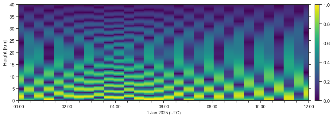
Rebin to new time bins
time_bin_centers = pd.date_range("20250101T00", "20250101T12", periods=30) # 30 instead of 300 time bins
p_rebinned_time_mean = p.rebin_time(time_bin_centers)
p_rebinned_time_interp = p.rebin_time(time_bin_centers, method="interpolate")
# Plotting
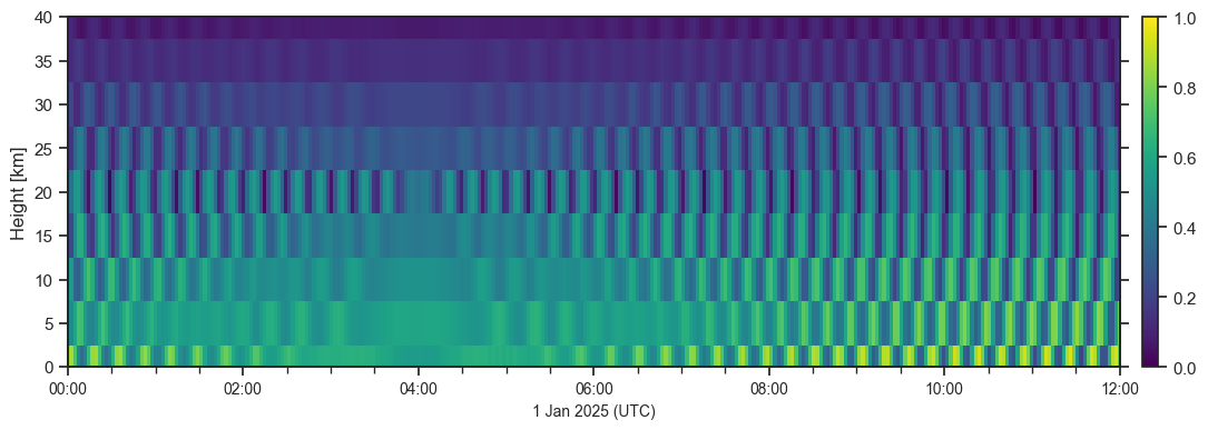
cf = eck.CurtainFigure().plot(p_rebinned_time_mean, value_range=(0,1))
cf.save(filepath="ts_rebin_time_mean_curtain.png")
cf = eck.CurtainFigure().plot(p_rebinned_time_interp, value_range=(0,1))
cf.save(filepath="ts_rebin_time_interp_curtain.png")
ts_rebin_time_mean_curtain.png |
ts_rebin_time_interp_curtain.png |
 |
 |